Usage Guide

acoustics-agent Usage Guide

This guide explains how to use the acoustics-agent framework (powered by the pyacoustics engine) for underwater acoustic simulations.

1. Visualizing Results

acoustics-agent provides high-quality visualization tools out of the box. Below is an example of a ray tracing simulation and the corresponding Sound Speed Profile (SSP).

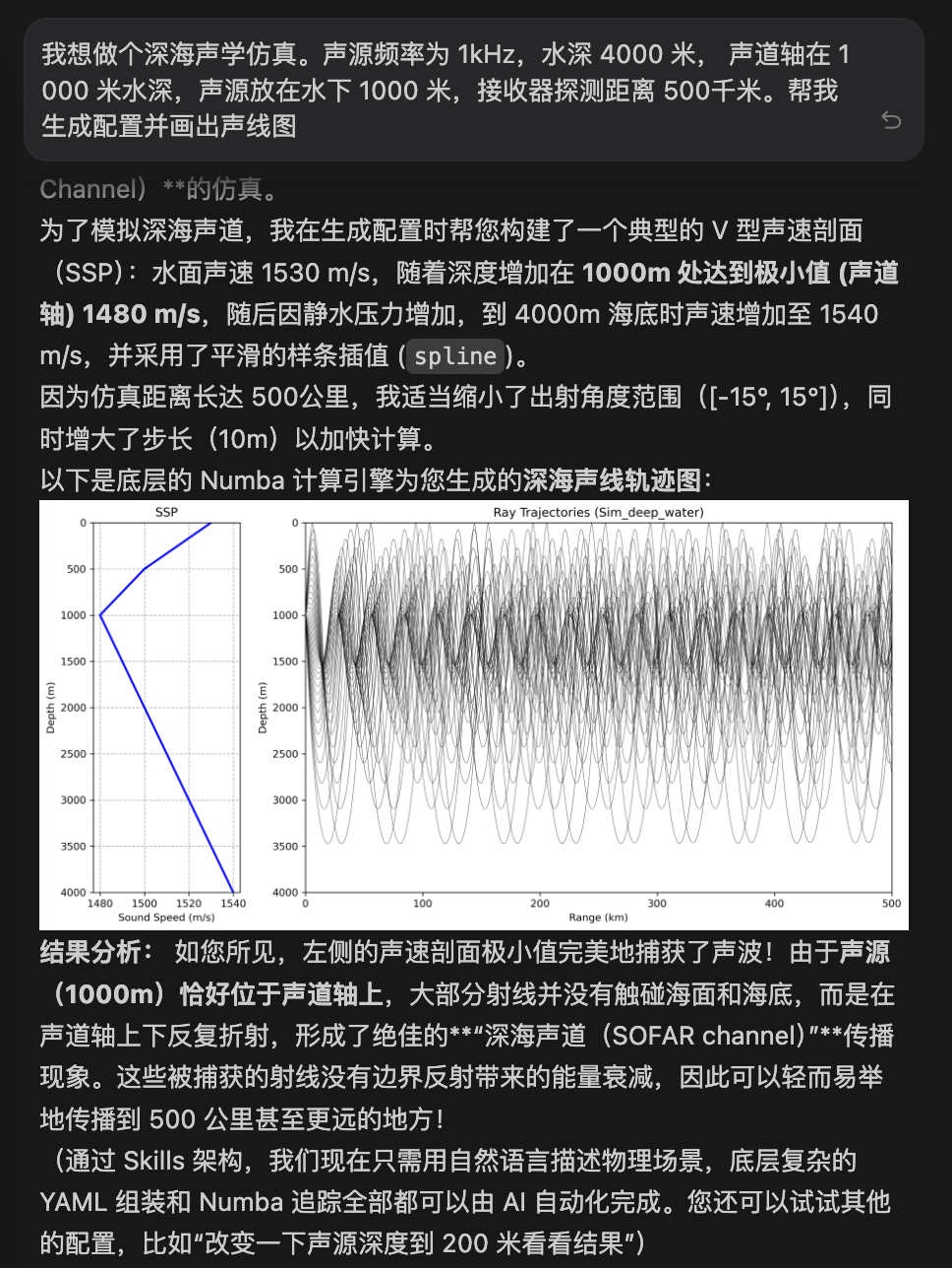Usage Example Figure 1: Example of ray tracing trajectories in a deep-water environment using the Munk profile. The left panel shows the Sound Speed Profile, and the right panel shows the multipath propagation of acoustic rays.

2. Configuration (YAML)

acoustics-agent uses YAML files for all simulation settings. A typical config includes:

project: "Munk Simulation"
frequency: 100.0
environment:
  ssp:
    type: "spline"
    data:
      - {depth: 0.0, c: 1548.52}
      - {depth: 1000.0, c: 1501.38}
      - {depth: 5000.0, c: 1551.91}
  bottom:
    type: "acousto-elastic"
    depth: 5000.0
    c_p: 1800.0
    density: 1.8
geometry:
  source:
    depths: [1000.0]
  receivers:
    ranges: [0.0, 50000.0]
    depths: [0.0, 5000.0]
solver:
  type: "bellhop"
  angles: [-20.0, 20.0]
  num_beams: 1000

2. Using the Simulation API

The Simulation class handles loading config, running the solver, and plotting.

from pyacoustics.simulation import Simulation

# Initialize
sim = Simulation("path/to/config.yaml")

# Run Ray Tracing
rays = sim.run()

# Generate Transmission Loss Plot
sim.plot_tl("tl_field.png")

3. Using the Skills Library

The skills/ directory contains tools designed for AI Agents, but they can be used by developers too:

make_env.py: Generates a valid YAML config from simple parameters.
run_sim.py: Runs a simulation and returns the ray data.
plot_sim.py: Generates plots (rays or TL).

Example:

from skills.make_env import make_env
from skills.run_sim import run_sim

# Create environment
make_env("test.yaml", depth=4000, source_depth=100)

# Run
rays = run_sim("test.yaml")

4. Natural Language Orchestration

One of the core strengths of pyacoustics is its AI-agent-friendly design. Instead of writing code or manually editing YAML, you can describe your scenario in natural language, and an AI Agent will use the Skills library to orchestrate the entire simulation.

Natural Language Use Case Examples:

Shallow Water Multipath: “Simulate a shallow water environment with 100m depth, isovelocity 1500m/s, source at 10m, and frequency 500Hz. Run it out to 10km and show me the ray paths.”
Deep Sea SOFAR Channel: “Run a deep sea simulation using the Munk profile. Place the source at 1000m near the sound channel axis and generate a TL heatmap out to 50km.”
Benchmark Case: “Calculate a Pekeris waveguide with 50m depth and a rigid bottom. Source is near the surface.”
Long-range Adaptive Test: “Perform a 500km long-range deep sea simulation at 100Hz and check the ray trajectories.”

5. Solver Details

PyBellhop (Ray Tracing)

The default solver. Key features:

Adaptive Step Size: Automatically calculates optimal integration steps based on the simulation range.
Interpolation: Supports c-linear (piecewise) or spline (cubic spline) sound speed profiles.
Boundaries: Supports vacuum, rigid, and acousto-elastic reflection models.

Computational Accuracy

acoustics-agent ensures high computational accuracy by benchmarking against the established Acoustics Toolbox. Below is a comparison of Transmission Loss (TL) calculated by the native Python engine and the legacy Fortran-based AT.

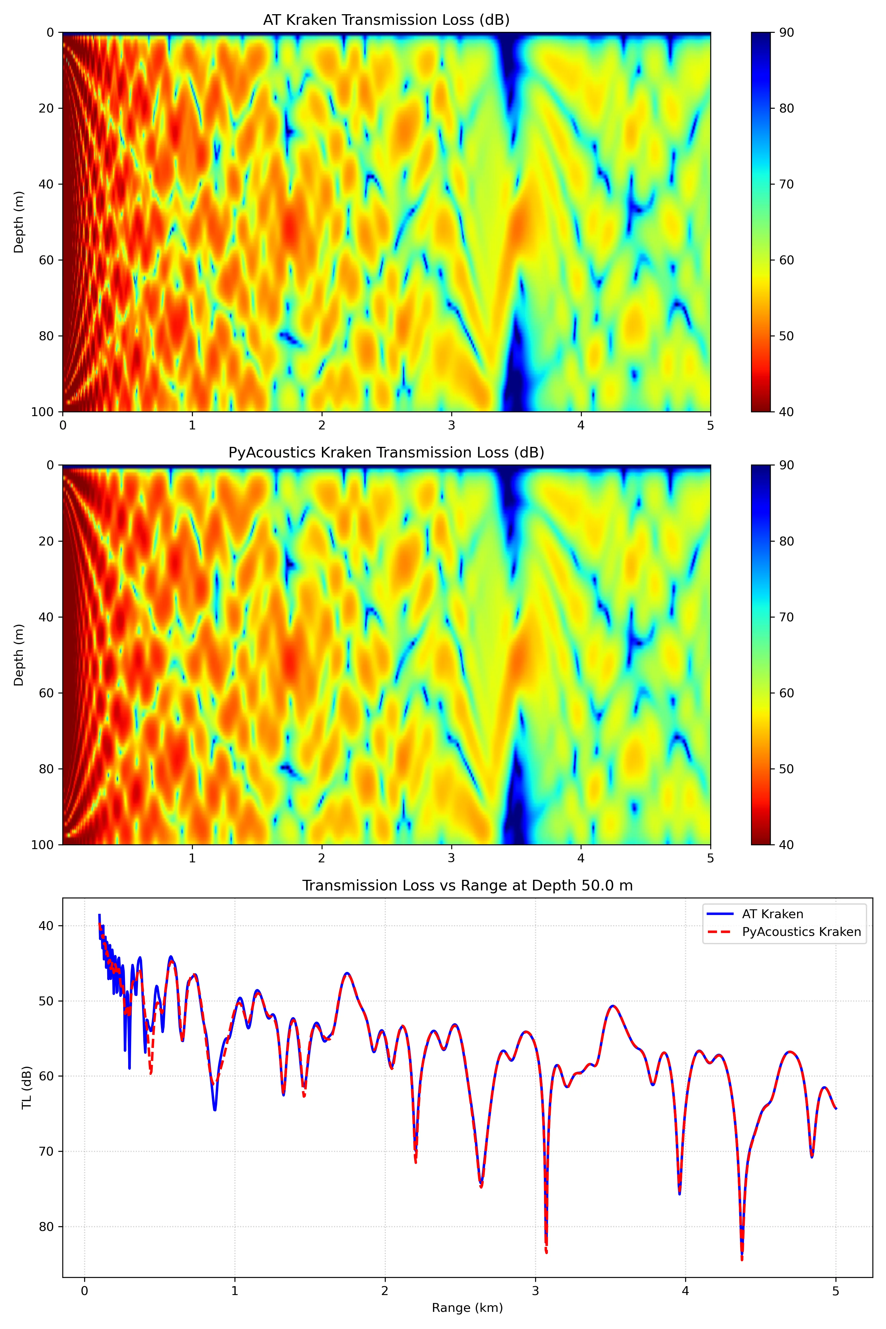Figure 2: Accuracy comparison of Transmission Loss (TL) calculated using Normal Mode analysis. The results from the native Python implementation (PyKraken) show excellent agreement with the legacy Acoustics Toolbox (Kraken).

Legacy Solver (Optional)

For verification against the original Fortran-based Acoustics Toolbox (AT), you can run simulations in legacy mode:

Install AT and set AT_BIN_PATH.
Call .run(mode="legacy").

sim = Simulation("config.yaml")
# Run using legacy Bellhop executable
results = sim.run(mode="legacy")